Chapter 33 - Fine, I’ll talk about AI #
[TODO] https://www.asimovinstitute.org/author/fjodorvanveen/
[TODO] https://playground.tensorflow.org/
Machine Learning? #
You’ve used it today. ML is used for search engines, social media feed order (the almighty Algorithm), and predictive text systems.
What is the difference between ML and AI? [TODO]
Learning is not the same as memorization, for example, if a baby sees his mother from various angles and under different lighting, he’s not memorizing her face. He’s learning features about it, which is why he can still recognize her in new views. Checking if two things are identical (or nearly so) is much easier, learning features and detecting things based on them is more difficult for a computer.
When to use ML?
- Computer being put in a situation where human’s have no direct experience
- No way to tell computer the human experience (speech recognition, facial recognition, driving)
- When the solution changes based on conditions/time (Driving in different weather / lighting, background noise removal)
- Every application is a bit different (different voices need different recognition)
when not to use ML?
- When all cases can be covered by a traditional program
Before I try to poorly explain something that has been explained much better than I can via text, I recommend watching this 4-video series from 3Blue1Brown, it totals just a hair over an hour.
With 3B1B’s videos done, I think it’s useful to just be exposed to some terms in bulk and get a sort of high level overview of what’s going on. For that, I recommend just putting this video on 2x speed and digesting it as best you can. Don’t worry if something makes you go, “huh?” for now:
Supervised Vs. Unsupervised Learning #
Supervised Learning #
Given labeled examples with features described, like pictures of trucks and cars, labeled ’truck’ or ‘car’ and data fields for wheel count, color, etc. that are populated, the machine learning algorithm makes a model that will try to classify new inputs.
Features can be as simple as the individual pixel values in an image
Let C be the target function to be learned. Think of C as a function that takes the input example and outputs a label. The goal is to, given a training set $ \chi = {(x^t,y^t) }^N_{t=1}$ where $y^t=C(x^t)$, output a hypothesis h ∈H, that approximates C when classifying new input.
Each instance x represents a vector of features (attributes). For example, let each $x=(x_1,x_2)$ be a vector describing attributes of a guitar; $x_1 = \text{sting count}, x_2=\text{acoustic or electric}$, each label is binary (positive/negative, yes/no, 1/0, etc.) and contributes to whether or not it’s a 6-string acoustic guitar.
A learning algorithm uses train set χ and finds a hypothesis h∈H that approximates C
error (loss) of h
- Empirical error is a fraction of χ that h gets wrong
- Generation error is the probability that a new, randomly selected, instance is misclassified by h. This depends on the probability distribution over instances. Generalization error is much more important than Empirical - it’s better to have it perform well on new data than be great on the training data
- False Negatives (C-h) and False Positives (h-C)
Unsupervised Learning #
Same as above, but no labels. (Still features). For example, https://en.wikipedia.org/wiki/K-means_clustering or Hierarchical clustering https://en.wikipedia.org/wiki/Hierarchical_clustering
Semi-supervised learning #
a mix of some labeled data, and some unlabed.
Pretrain to get relevant features
transfer-learning, take training from one task and apply it to another (should this be here?)
Reinforcement Learning #
agent takes step, looks at environment, makes actions based on it, repeat. Goal it to maximize expected long term reward
Often used for games
Markov Decision Process
Sorta like a state machine
feedback is often delayed - credit assignment problem
How does it work? #
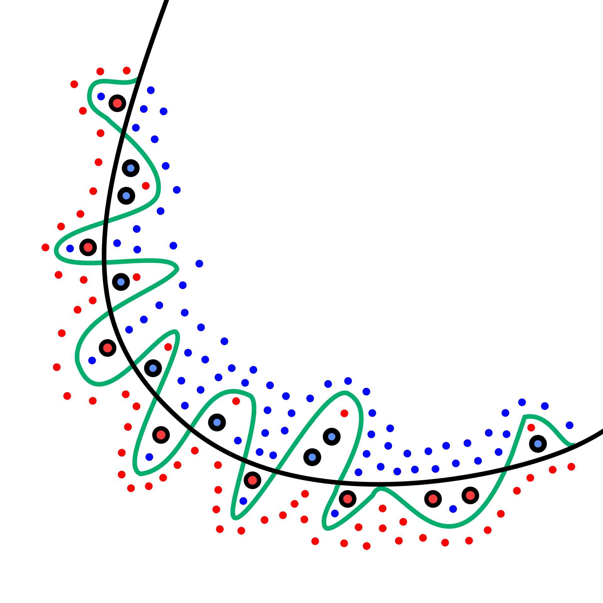
Not overfitting - spikey vs smooth curve. Spikey to directly fit is bad, similar with XY blobs with reaching out arms balance with model complexity with regulizer. We want generalization (learning) not memorization
Models #
Decision trees
support vector machines
probabilistic graphical models
Artificial Neural Networks -> Deep learning (many layers)
Each node multiplied by weight, sent though activation function, often using stochastic gradient descent
Performance Measures #
Classification error - fraction of time correct
Squared error
cross entropy
No single best approach
Linear Unit (Regression) #
[TODO] tie back to https://en.wikipedia.org/wiki/Linear_regression
a vector with features x_1 to x_2 and weights w_1 to w_n
 \(\hat{y}=f(x;w,b)=x w+b=w_1x_1+....w_nx_n+b\)
b can be represented as \(w_0\) instead, as is shown in the above
 \(y=o(x;w,b)=\{{+1 \text{ if } f(x;w,b)>0\atop{-1 \text{ otherwise}}}\)
(sometimes 0 instead of -1)
for binary classification, +1 is it is the thing, -1 (or 0) is saying it’s not the thing.
not all functions are linearly separable, one straight line can’t split the data into positives and negatives- so having networks of units works around this
Of course, we’d like to be able to use inputs that aren’t just numbers. Representing things like price or weight can be given a number, but for other things, like colors, one hot vectors are helpful, for example, if there are three color options, red, green, blue, red could be [1,0,0], green [0,1,0], blue [0,0,1]. This is better than just assigning each color an integer (red=1,green=2,blue=3, etc.) because we don’t want to imply ordering in the data. One hot vectors are especially nice because they let us assign positive weights to a given color and negative weights to others. For example, in identifying a fire truck, red will obviously have a very positive weight, while being the other colors may be a negative weight.
Training:
\(w_j\prime\larr w_j+\eta(y^t-\hat{y}^t)x^t_j\)\(w_j\prime\) is the new value of \(w_j\) , (the j’th w as each weight is incremented though)
\(x_j^t\) is the jth attribute of training instance t
\(y^t\) is the label of training instance t
\(\hat{y}^t\) is Perception output on training instance t
η > 0, the learning rate, is a small constant (e.g.; 0.1)
if \((y-\hat{y})>0 \text{ then increase } w_j \text{ w.r.t } x_j\) else decrease
Can prove rule will converge if training data is linearly separable and η sufficiently small
a bad learning rate, η, can cause very slow convergence (too small) or even divergence (too large)
It’s best to adjust the learning rate per schedule (iteration) rather than just use a constant. For this, we want to start with a high learning rate, then decrease it.
| Schedule | Formula |
|---|---|
| Power Scheduling | \(\eta(t)=\eta_0/(1+t/s)^c\) |
| Exponential Scheduling | \(\eta(t)=\eta_0(0.1)^{t/s}\) |
| Performance Scheduling | reduce η by λ when no improvement in validation |
| 1cycle Scheduling | increase from \(\eta_0 \text{ linearly to } \eta_1\) then back down to \(\eta_0\) |
Gradient Descent #
[TODO] https://en.wikipedia.org/wiki/Gradient_descent
[TODO] Stochastic Gradient Descent
momentum term β to keep updates moving in the same direction as previous trials
this can help move though local minima to a better local or global minimum and not get stuck on flat spots
Adagrad adapts learning rate by scaling it down in the steepest dimensions
RMSProp exponations decays old gradients to avoid AdaGrad’s problem of stopping too early for neural networks duo to aggressive downscaling
Adaptive Moment Estimation (Adam) combines momentum optimization and RMSProp
Nonlinearly separable Problems #
XOR
| Input A | Input B | Output |
|---|---|---|
| 0 | 0 | 0 |
| 0 | 1 | 1 |
| 1 | 0 | 1 |
| 1 | 1 | 0 |
No single linear threshold unit can describe this
in 2d a line, in 3d a plane, 4+d hyperplane
Every one side of these is a halfspace, but given two functions, we can get an overlap, the intersection of the two halfspaces
now, we can find $z_i$ , mapping though a non-linear function, from x space to z space, now the problem is linearly separable- there’s no need for the dimensions from mapping from x-to-z space to be the same, and there can be multiple hidden layers
We’ve mapped from a non-linearly separable problem into a linearly separable one
Feedforward Neural Networks on Wikipedia
generally, if the input can be split up with straight lines and be defined as the unions and intersections of those halfspaces, then two hidden layers and an output layer must exist that works
Backpropagation #
First, feed forward the network’s inputs to its outputs, then propagates back error with by repeatedly applying the chain rule
propagate error back in order to compute loss gradient with respect to each weight, then update the wights
don’t have to update the loss on each instance, could do mini-batches (Stochastic Gradient Descent- SGD), or in the extreme case, have the entire training set be a single batch (batch gradient descent). SGD saves on memory, which helps.
Computation Graphs #
(note the library- tensor flow, pytorch, etc.- will probably handle this for you)
given a complicated function, we want to know its partial derivatives with respect to its parameters
For
multivariate chain rule, multiple paths that can affect the output. Math gets very gross very quickly
The Sigmoid Unit #
$S(x)=\frac{1}{1+e^{-x}}$ squashes everything into a range from 0 to 1 (or -1 to 1), with 0 mapping to ½. It’s similar to the threshold function, for us, this is useful as $\sigma(x)=\frac{1}{1+e^{-net}}$, where $net=\sum_{i=0}^{n} w_i x_i=f(x;w,b)$

Types of Output Units #
Linear - works well with GD training
Logistic - good for probabilities
Softmax - every output node
Types of Hidden Units #
Logistic - has issues with saturation
Rectified Linear Unit (ReLU)
leaky ReLU and exp ReLU
How many layers to use? #
Increasing number of layers increases risk of overfitting, need more training data for deeper network to avoid this
performance improvement even without more parameters
Gotta know when to add more layers instead of parameters, but in general adding more layers is better, that is try adding layers before widening, keeping in mind the overfitting problem. Also, increases training time
ANN - Artificial Neural Networks #
Silicon ’neurons’ are much faster, but connect to many fewer nodes, compared
[TODO] get human neuron count, ‘switching time’, interconnectivity
much different for ML vs Biological Modeling
think a ton of really weak cores, which explains the GPU usage
good for raw sensor data, okay with noise, but requires long training times and lacks human readability- hard to know why it predicts what it does
Started with the Perceptron algorithm, but that was too limited (40’s)
multi-layer backpropagation (80’s) allowed for training multi layer networks, and they couldn’t be made deep on that era’s hardware, while other algorithms (Support Vector Machines, boosting) were taking off instead. In the 2000s it became possible for 5-8 layers though, making ‘deep’ learning possible (mostly because of gaming GPUs). Better datasets, and better algorithms, helped too.
Any boolean function can be represented with 2 layers
any bounded continuous function can be represented with arbitrarily small error with two layers
that goes to any function at 3 layers
but, this is only true for existence. It may be very, very difficult to find the weights and take a ton of nodes
Initialization #
We used to initialize parameters to random numbers near 0, but now Glorot is used,
with $n_{in} \text{ inputs and } n_{out} \text{ outputs}$, initialize with a uniform from $[-r,r]$ with $r=a\sqrt{\frac{6}{n_{in}+n_{out}}}$ or normal, $\mathcal{N}(0,\sigma)$, with $\sigma=a\sqrt{\frac{2}{n_{in}+n_{out}}}$
| Activation | a |
|---|---|
| Logistic | 1 |
| tanh | 4 |
| ReLU | √2 |
Gradient Descent #
alt: evolution
Nonlinearly separable problems and multilayer networks #
Types of Activation Functions #
Convolutional Neural Networks #
Good for data with grid/array like topology, think images or time series data
based on using convolutions and pooling- extract features, invariant to transforms, parameter efficient
passing a kernel over an image, just doing a sliding window, like normal - can do edge detection, blurring, etc.
Kernels are just weights, so, we can learn the best weight to use
not complete connectivity, that is no crossing from layer to another, the layer above only depends on one path
… unless we use a convolutional stack(?)
… next node over probably shares many parameters (weight sharing), the computation graph could just share this overlap to reduce parameters. Saves memory
weight sharing forces the layer to learn a specific feature extractor. Multiple layers could be learned in parallel, as only detecting one feature (like vertical lines) may not be helpful.
on images this is commonly done as separate detectors on color channels and multiple for specific feasters. Each higher layer is for a more complex feature, with multiple channels of features.
Basically,
can pad to retain size, 0-padding is common
can use a stride-parameter to downsample

pooling nodes help get translation invariance
Downsides of CNNs: Many parameters to tune, large memory usage
often better to modify a prior network trained on a bigger dataset and for longer - Transfer Learning
Object Detection can look for local areas of interest:
R-CNN, SPP-NET, Fast R-CNN, YOLO - You Only Look Once
Regularization and Evaluation #
ML is basically an optimization problem
We need a function to measure performance - a loss function
Given instance x, with label y, and a prediction $\hat{y}$, then $J(y,\hat{y})$ is the loss on that instance
| Function | Common Use | Formula |
|---|---|---|
| 0-1 Loss | $J(y,\hat{y})=1$ if $y\neq\hat{y}$, 0 otherwise | |
| Square Loss | Regression | $J(y,\hat{y}) = (y - \hat{y})^2$ |
| Cross-Entropy | y and $\hat{y}$ are considered probabilities of a ‘1’ label. Allows for two probability distributions. Good for when the input data also has probability. Often used for classifying images | $J(y,\hat{y})$ = $(-y)ln(\hat{y})-(1-y)ln(1-\hat{y})$ |
| Hinge Loss | Large Margin Classifier | $J(y,\hat{y}) = max(0,1-y\hat{y})$ |
given a loss function, J, and a dataset, X, $error_x(h)=\sum_{x\in h}J(y_x,\hat{y}_x)$ where $y_x$ is x’s label, and $\hat{y}_x$ is h’s prediction
But, it’s more important that the model generalizes, so given a new example (picked i.i.d) according to unknown probability distribution D, we want to minimize h’s expected loss $error_D(h)=\mathbb{E}_{x\sim{D}}[J(y_x,\hat{y}_x)]$
minimizing training loss isn’t the same as minimizing expected loss? NO
By doing to good on the training set, the over fitting will make results pretty bad. That is a specific parameter h overfits the training data, X, if there is an alternative hypothesis, $h^\prime$ such that $error_x(h) < error_x(h^{\prime})$ and $error_D(h) > error_D(h^{\prime})$
This is literally just the formal defn’ of overfitting. Don’t over think it.
Overfitting example by Chabacano - CC BY-SA 4.0
Note that underfitting is just as much of a problem. Training accuracy needs to be balanced with simplicity.
Overfitting is often a result of an overkill network topology, training too long, not having enough training data, or not doing early stopping.
Complexity Penalty $J^{\sim}(\theta;X,y)=J(\theta,X,y)+\alpha\Omega(\theta)$ where $\alpha \in [0,\infin)$ weights loss J against penalty $\Omega$. $\Omega(\theta)$ just measures complexity via $\Omega(\theta)=(0.5)||\theta||_2^2$, that is the sum of the squares of network’s weights. Since $\theta=w$, this becomes
$J^{\sim}(w;X,y)=(\alpha/2)w^{\top}w+J(w;X,y)$
as weights deviate from 0, activation functions become more nonlinear, which brings a higher risk of overfitting
Early Stopping #
danger of stopping too soon, as it might just have a ‘bump’
Data Augmentation #
Careful not to change class- ie 6 → 9 or E → 3 in images
protects against translation/rotation and overfitting/underfitting
adding noise
Multitask Learning #
Share common layers of lower network
Dropout #
Prevents any node from becoming too specialized sorta distributes the work load
Batch Normalization #
Parameter Tying #
Parameter Sharing #
Sparse Representations #
Other Resources #
Academic #
i.am.ai Roadmap - a ‘Roadmap’ to learning AI
https://hific.github.io - Image compression with GANs
Insipriational & Artistic #
The Art of Asking Nicely (AI Weirdness)
ML model can classify sex from retinal photograph, clinicians can’t
Darknet - an open source neural network framework written in C and CUDA, with lots of examples