9 - Probability/Stats #

Seeing Theory: A visual Introduction to probability and statistics

Why, where are these used, etc.

bring up music things, part failure rates, tolerances, etc.

Basics #

For the following, I’ll be using a die roll example, where the events are the total of two die. The Sample Space of this is

Note, that 1 isn’t possible as the lowest is both die being ‘1’.

Let’s look at the probability of these outcomes,

While there are 11 (2-12) unique outcomes, there are 36 possible outcomes from the two die, which are shown in the table above.

If you follow the diagonal you can see that there is only one way to get 2 or 12, two ways to get 3 or 11, and so on, this gives this table:

Now, let’s say we want the probability that we roll an even total (2,4,6,8,10,12) we can just sum their respective probabilities, so \(\frac{1}{36}+\frac{3}{36}+\frac{5}{36}+\frac{5}{36}+\frac{3}{36}+\frac{1}{36} = \frac{18}{36} = \frac{1}{2}\)

Let’s go ahead and call this event A, so P[A] = 1/2

Similarly, we can define a new rule, Event B, such that the roll total is greater than 9, that comes out to be 1/6, so P[B]=1/6

Statistical Independence #

Event A and event B are statistically independent if and only if (iff) \( P[AB] = P[A]P[B]\)

So, here, P[AB], that is the probability that a number is both greater than 9 and the number is even, that would be 1/9. The probability of each event multiplied together, \(P[A]P[B] = \frac{1}{2} * \frac{1}{6} = \frac{1}{54}\) and, hopefully obviously, that’s not the same as 1/9. Therefore, these events are not statistically independent. This makes logical sense, if you know that the total count of the two die is greater than 9, then you also know that there’s a higher chance that the result is even - of 10,11, and 12, 2/3 of the totals are even. That is dependence.

If instead, we asked, what is the probability that 1 die is a 6 and the other a 2, both of those would have a probability of 1/6, that is \(P[A]=P[B]=\frac{1}{6} \) , so now think, in the combined scenario, P[AB] would be the probability of die 1 being a 6, and die 2 being a 2, well, there are 36 different ways the die can land, and they’re all unique (assuming the die are labeled somehow) so \(P[AB]=\frac{1}{36} = P[A]P[B] \) - these events are statistically independent.

It’s worth noting, the physical relationship is not always this clear. In a lot of situations, you’ll just need to do the math and determine if \(P[AB] = P[A]P[B]\) to check.

Conditional Probability #

Sometimes, knowing something about one event tells us something about the probability of another event. This can be expressed mathematically. When written down, it looks a bit gross, but it’s actually really easy to understand:

This also provides another equation, just by moving things around:
\(P[A|B]=\frac{P[AB]}{P[B]} \)

Here, P[A|B] means, the probability of event A happening given event B has already happened.

So, looking at just one side of the above equation, we have \(P[A|B]P[B]=P[AB]\) , this reads as “The Probability of A given that B has happened times the Probability of B is equal to the probability of an event that is in both A and B”

The other side of this equation, is just swapping the roles of A and B.

So, let’s go off the above example and assume that you’re really bad at showing up for work:

So shoving these values in to the above, we can determine that

So, if you lose your keys, you’ll be late to work 1/3rd of the time.

Alright, but what about a more complicated situation, one where you have to make multiple decisions! Let’s

Keeping the numbers simple here, let’s say you want to know the probability that the ball you picked was from box1, given that you’ve already drawn a blue ball. This is where a Tree diagram comes in handy:

This diagram first helps us expose an assumption in the problem: that the initial choice is a 50/50, split chance between which box we start with. So our first choice is really which box are we picking from. Both have a probability of 1/2. Only then do we pick our ball. This stacking of situations gives us the term ‘sub experiment’ where you perform each sub experiment in order: so our first sub experiment is picking the box, the second is picking the ball.

This lets us figure out the conditional probabilities super easily, as all that’s needed is to look at the respective branch. For example, in the above, we can see P[Red|Box1] is 9/10. Another nice thing is by multiplying across the branches we can get the probability of the entire ‘system’ easily. Note the ‘,’ instead of a ‘|’ in the diagram below. This is saying that these have both happened, not implying conditional probability. That’s why adding all of these up will add up to 1 (100%) as it’s a look at all the possible events.

So now we know the probability of a blue ball overall: 0.4 (.05 + .35 )(1), the probability of a blue ball in box 1 (.1), what is the probability that we actually picked from box 1? We know P[Blue|Box1], but what is P[Box1|Blue] ? Well, naturally, there’s a handy formula, known as “Bayes Rule” for this situation:

[TODO] Why Bayes Rule is nicer with odds (YouTube, 3b1b)

Applying this, we can see that we get

so, there’s a 12.5% chance that the box we picked the blue ball from was Box1.

Just to check ourselves, what’s the chance that the box was Box2?

And this works out, adding to 100%.

There are a few more things to note regarding conditional probability:

• if P[A|B] is 0, the two events are mutually exclusive. This happens in dumb situations like “Given you’ve rolled a 2, what is the probability you rolled a 3” but also more complex events may mean that this is less obvious, so it’s nice to be able to math it out.

[TODO]

Tree diagram with more branches, some ‘incomplete branches’

fair/unfair coin:

/C1-H-H-H \C2-H-H-H

Sub experiments & Tree diagrams

Counting methods

combinations and permutations

Looking at binary, arrangements of bits

with or without replacement

Random Variables #

Probability Mass Function (PMF)

Types of RV’s

[TODO] http://www.math.wm.edu/~leemis/chart/UDR/UDR.html

Bernoulli #

Geometric #

Original Image by Skbkekas - Own work, CC BY 3.0, link

In probability theory and statistics, the geometric distribution is either one of two discrete probability distributions:

• The probability distribution of the number X of Bernoulli trials needed to get one success, supported on the set { 1, 2, 3, … }

• The probability distribution of the number Y = X − 1 of failures before the first success, supported on the set { 0, 1, 2, 3, … }

Which of these one calls “the” geometric distribution is a matter of convention and convenience.

- Wikipedia

Binomial #

Original Image by Tayste - Own work, Public Domain, link

Sum of n, independent Bernoulli trials

Pascal (Negative Binomial) #

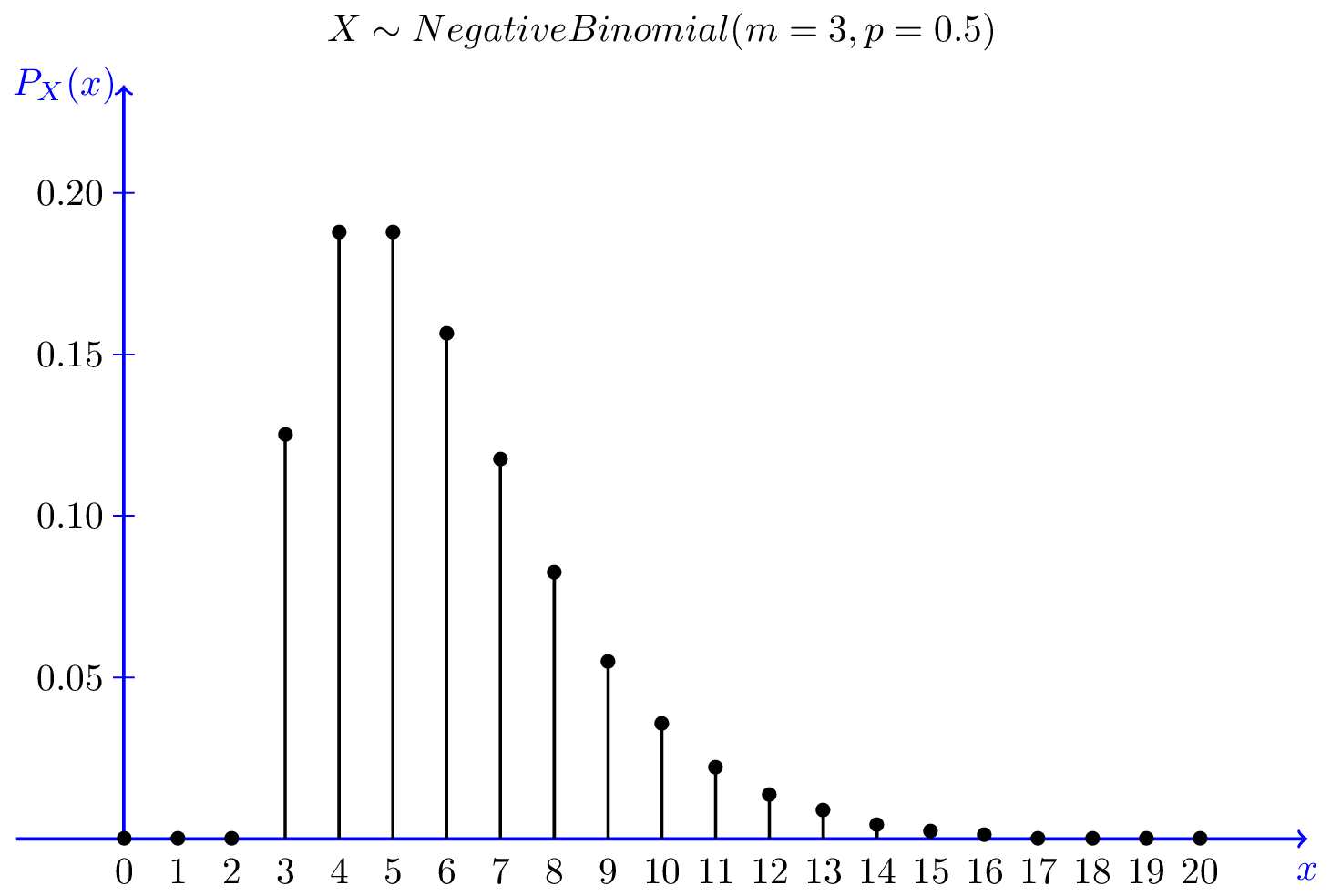
From Introduction to Probability by Hossein Pishro-Nik, CC BY-NC-ND 3.0 … technically I’m abusing the license a bit, but the ‘derivative’ here is just a CSS invert, you can open the image in a new tab to see the ‘original’

Number of trials until k’th success. While technically the Pascal distribution is just a specific subset of Negative Binomial distributions, you’ll probably only ever use the Pascal distribution. Be aware the more general case exists, though, as someday it may pop up.

Discrete Uniform #

Original Image by IkamusumeFan - Own work, CC BY-SA 3.0, link

It’s a uniform distribution. Rolling a fair dice? Great, you have 1/6 chance to get a 1,2,3,4,5, or 6. So your ‘a’ and ‘b’ are 1 and 6, ’n’ is the number of points, so b-a+1

Poisson #

Original Image by Skbkekas - Own work, CC BY 3.0, link

Probability of a number of events occurring in a fixed amount of time (or space, or whatever) provided the events happen with a constant average rate and the events are independent.

Cumulative Distribution Function (CDF)

functions of Random Variables

Families of continuous RVs

Conditional Probability Mass Fn & Conditional Expected Value

Gaussian Random Variables / Normal RVs (same thing)

Cheatsheet and another one

[TODO] Gaussian Processes From Scratch (Peter Rlnts)

[TODO] https://mc-stan.org/users/documentation/

[TODO] The Fisher Information (YouTube - Mutual Information)

Chaos #

1. Technically, this is the "Law Of Total Probability". Don't overthink this. It just means that by adding up all the conditional probalities of a certain event, you get the total probability. Here, we're adding up the probability of a blue ball given we picked box1 AND the probability of a blue ball given we picked box 2. It's sorta obvious this would give us the total probability of a blue ball.